Parallel Reduced Ion Distribution and Fit

author: Louis Richard

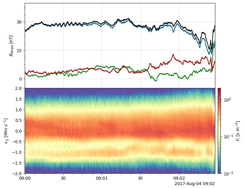
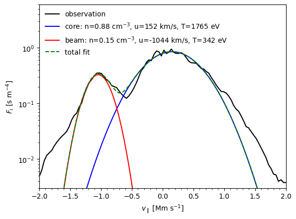
Computes the reduced ion velocity distribution function \(f_i(v_\parallel)\) along the FGM magnetic field from FPI burst-mode skymaps with Monte-Carlo integration (mms.reduce), using the EDP spacecraft potential, and plots it as a time series. It then fits a two-component (core and beam) Maxwellian model to the distribution at a selected time with scipy.optimize.curve_fit.

%matplotlib inline

import matplotlib.pyplot as plt
import numpy as np

from pyrfu import mms, pyrf
from pyrfu.plot import use_pyrfu_style, plot_spectr, plot_line

use_pyrfu_style(usetex=False)

Load data

Define time interval and spacecraft index

mms.db_init(default="local", local="/data/mms")
tint = ["2017-08-04T09:00:00", "2017-08-04T09:02:28"]
mms_id = 1

[05-Oct-26 18:04:35] INFO: Updating MMS data access configuration in /homelocal/louisr/.config/pyrfu/mms_config.json...
[05-Oct-26 18:04:35] WARNING: No system keyring available: MMS SDC credentials saved in plain text in /homelocal/louisr/.local/share/python_keyring/keyring_pass.cfg

Load the magnetic field

b_dmpa = mms.get_data("b_dmpa_fgm_brst_l2", tint, mms_id)

[05-Oct-26 18:04:35] INFO: Loading mms1_fgm_b_dmpa_brst_l2...

sc_pot = mms.get_data("v_edp_brst_l2", tint, mms_id)

[05-Oct-26 18:04:36] INFO: Loading mms1_edp_scpot_brst_l2...

Load the spacecraft attitude

Used to convert between Geocentric Solar Ecliptic (GSE) and spacecraft coordinates.

defatt = mms.load_ancillary("defatt", tint, mms_id)

[05-Oct-26 18:04:37] INFO: Loading ancillary defatt files...

Load the ion VDF skymaps and their uncertainties

The uncertainty is \(\delta f / f = 1/\sqrt{n}\), with \(n\) the number of counts.

vdf_i = mms.get_data("pdi_fpi_brst_l2", tint, mms_id)
vdf_i_err = mms.get_data("pderri_fpi_brst_l2", tint, mms_id)

[05-Oct-26 18:04:44] INFO: Loading mms1_dis_dist_brst...
[05-Oct-26 18:04:45] INFO: Loading mms1_dis_disterr_brst...

Define the coordinate system of the projection

• \(x\) is along the local magnetic field.

• \(y\) and \(z\) are perpendicular to \(x\), with \(z\) as close as possible to the spacecraft spin axis.

x_hat = pyrf.resample(b_dmpa, vdf_i)
x_hat.data /= pyrf.norm(x_hat).data[:, np.newaxis]
z_hat = pyrf.ts_vec_xyz(
    vdf_i.time.data, np.array([0, 0, 1]) * np.ones((len(vdf_i.time), 3))
)
y_hat = pyrf.cross(z_hat, x_hat)
y_hat.data /= pyrf.norm(y_hat).data[:, np.newaxis]
z_hat = pyrf.cross(x_hat, y_hat)
z_hat.data /= pyrf.norm(z_hat).data[:, np.newaxis]

xyz = np.transpose(np.stack([x_hat.data, y_hat.data, z_hat.data]), [1, 2, 0])
xyz = pyrf.ts_tensor_xyz(vdf_i.time.data, xyz)

Define the velocity grid along the magnetic field

vpara_lim = np.array([-2e3, 2e3], dtype=np.float64)
vg_para = np.linspace(vpara_lim[0], vpara_lim[1], 100)

Reduce the distribution along the magnetic field

f1dpara = mms.reduce(
    vdf_i,
    dim="1d",
    xyz=xyz,
    n_mc=200,
    vg=vg_para * 1e3,
    lower_e_lim=30.0,
    sc_pot=sc_pot,
)
f1dpara = f1dpara.assign_coords(vx=f1dpara.vx.data / 1e3)

100%|█████████████████████| 987/987 [00:14<00:00, 69.75it/s]

Plot

f, axs = plt.subplots(2, sharex="all", figsize=(9, 6.5))
f.subplots_adjust(hspace=0.0, left=0.15, right=0.85, bottom=0.08, top=0.95)
plot_line(axs[0], b_dmpa)
plot_line(axs[0], pyrf.norm(b_dmpa), color="k")
axs[0].set_ylim([-5, 40])
axs[0].set_ylabel("$B_{dmpa}~[\mathrm{nT}]$")

axs[1], cax1 = plot_spectr(
    axs[1], f1dpara, cscale="log", clim=[1e-2, 2e0], cmap="Spectral_r"
)
axs[1].set_ylim([-2, 2])
axs[1].set_ylabel("$v_\\parallel~[\\mathrm{Mm}~\\mathrm{s}^{-1}]$")
cax1.set_ylabel("$F_i~[\\mathrm{s}~\\mathrm{m}^{-4}]$")

axs[-1].set_xlim(pyrf.iso86012datetime64(np.array(tint)))

<>:6: SyntaxWarning: invalid escape sequence '\m'
<>:6: SyntaxWarning: invalid escape sequence '\m'
/tmp/ipykernel_523407/2824225912.py:6: SyntaxWarning: invalid escape sequence '\m'
  axs[0].set_ylabel("$B_{dmpa}~[\mathrm{nT}]$")

(np.float64(17382.375), np.float64(17382.376712962963))

Fit and plot a 1D reduced distribution

Select the ion distribution at a given time

t_sel = np.datetime64("2017-08-04T09:01:08.105711000")
f1dpara_sel = f1dpara.sel(time=t_sel)

Define the Maxwellian and two-component models

from scipy import constants, optimize

# Define the Maxwellian distribution function


def maxwellian(v, n, u, t):
    m_i = constants.proton_mass
    v_th = np.sqrt(2 * constants.electron_volt * t / m_i)
    coeff = n / (np.sqrt(np.pi) * v_th)
    exponent = -((v - u) ** 2) / v_th**2
    return coeff * np.exp(exponent)


# Define the two-component Maxwellian model


def two_components(v, n1, u1, t1, n2, u2, t2):
    return maxwellian(v, n1, u1, t1) + maxwellian(v, n2, u2, t2)

Fit the reduced distribution

# Fit the two-component Maxwellian model to the data
popt, _ = optimize.curve_fit(
    two_components,
    f1dpara.vx.data * 1e6,
    f1dpara.data[454, :],
    p0=[0.2e6, -1100e3, 520, 1e6, 100e3, 1700],
)

# Compute the fitted components
core = maxwellian(f1dpara.vx.data * 1e6, *popt[3:])
beam = maxwellian(f1dpara.vx.data * 1e6, *popt[:3])
tota = two_components(f1dpara.vx.data * 1e6, *popt)

Plot the fit

f, ax = plt.subplots(1)
ax.semilogy(f1dpara.vx.data, f1dpara.data[454, :], color="k", label="observation")

ax.semilogy(
    f1dpara.vx.data,
    core,
    color="b",
    label=f"core: n={popt[3]*1e-6:.2f} cm$^{{-3}}$, u={popt[4]*1e-3:.0f} km/s, T={popt[5]:.0f} eV",
)
ax.semilogy(
    f1dpara.vx.data,
    beam,
    color="r",
    label=f"beam: n={popt[0]*1e-6:.2f} cm$^{{-3}}$, u={popt[1]*1e-3:.0f} km/s, T={popt[2]:.0f} eV",
)
ax.semilogy(f1dpara.vx.data, tota, color="g", linestyle="--", label="total fit")

ax.set_ylim([3e-3, 6e0])
ax.set_xlim([-2, 2])
ax.set_xlabel(r"$v_\parallel~[\mathrm{Mm}~\mathrm{s}^{-1}]$")
ax.set_ylabel(r"$F_i~[\mathrm{s}~\mathrm{m}^{-4}]$")

ax.legend(loc="upper left")

<matplotlib.legend.Legend at 0x719a8814dfd0>