Electron Diffusion Region Signatures#
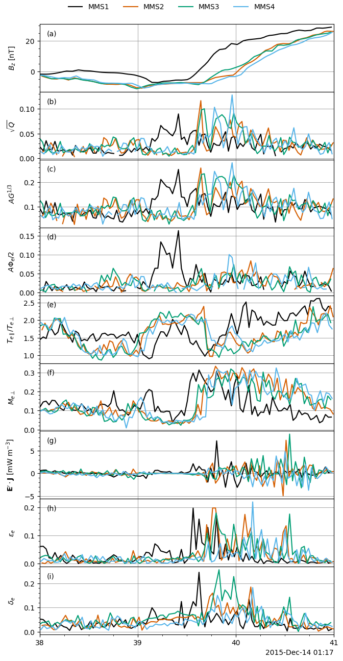
The quantities computed so far are: - \(\sqrt{Q}\) (Swisdak, 2016): values around 0.1 indicate electron agyrotropy. Computed from the off-diagonal terms of the pressure tensor for \(P_{e\perp 1} = P_{e\perp 2}\).
\(D_{ng}\) (Aunai et al., 2013): computed from the off-diagonal terms of the pressure tensor for \(P_{e\perp 1} = P_{e\perp 2}\). Similar to \(\sqrt{Q}\) but with a different normalization. Computed but not plotted.
\(AG^{1/3}\) (Che et al., 2018): constructed from the determinant of the electron pressure tensor rotated into field-aligned coordinates (\(P_{e\perp 1} = P_{e\perp 2}\)).
\(A\Phi_e/2 = |P_{\perp 1} - P_{\perp 2}|/(P_{\perp 1} + P_{\perp 2})\): a measure of electron agyrotropy. Values of \(O(1)\) are expected in EDRs. The pressure tensor is rotated into field-aligned coordinates such that the difference between \(P_{e\perp 1}\) and \(P_{e\perp 2}\) is maximal, which corresponds to \(P_{23} = 0\). (This definition of agyrotropy neglects the off-diagonal pressure terms \(P_{12}\) and \(P_{13}\), so it does not capture all agyrotropies.)
\(A_{n_e} = T_\parallel/T_\perp\): values much larger than 1 are expected. Large \(T_\parallel/T_\perp\) is a feature of the ion diffusion region (IDR). For magnetopause reconnection, MMS observations give \(A_{n_e} \sim 3\) in ion diffusion regions. Scudder gives \(A_{n_e} \sim 7\) at the IDR–EDR boundary, but this is extremely large for magnetopause reconnection.
\(M_{e\perp}\): electron Mach number, i.e., the bulk velocity divided by the electron thermal speed perpendicular to \(\mathbf{B}\). Values of \(O(1)\) are expected in EDRs (Scudder et al., 2012, 2015).
\(\mathbf{J}\cdot\mathbf{E}'\): \(\mathbf{J}\cdot\mathbf{E}' > 0\) is expected in the EDR and corresponds to the dissipation of field energy. \(\mathbf{J}\) is computed on each spacecraft from the particle moments (Zenitani et al., 2011).
\(\epsilon_e\): energy gain per cyclotron period. Values of \(O(1)\) are expected in EDRs (Scudder et al., 2012, 2015).
\(\delta_e\): relative strength of the electric and magnetic forces in the electron bulk rest frame. N.B.: very sensitive to the electron moments and the electric field; check the version of these quantities (Scudder et al., 2012, 2015).
Notes: \(\kappa_e\) (not yet included) is taken to be the largest value of \(\epsilon_e\) and \(\delta_e\) at any given point. Requires electron distributions with version number v2.0.0 or higher. The agyrotropy measures (1)–(3) become unreliable at low densities, \(n_e \lesssim 2~\mathrm{cm}^{-3}\), when the raw particle counts are low. Agyrotropies are removed for \(n_e < 1~\mathrm{cm}^{-3}\).
[1]:
%matplotlib inline
import numpy as np
import matplotlib.pyplot as plt

from pyrfu import mms, pyrf
from pyrfu.plot import use_pyrfu_style, make_labels, pl_tx
from scipy import constants

use_pyrfu_style(usetex=False)
Define time interval and data path#
[2]:
mms.db_init(default="local", local="/data/mms")
tint = ["2015-12-14T01:17:38.000", "2015-12-14T01:17:41.000"]
[05-Oct-26 17:39:47] INFO: Updating MMS data access configuration in /homelocal/louisr/.config/pyrfu/mms_config.json...
[05-Oct-26 17:39:47] WARNING: No system keyring available: MMS SDC credentials saved in plain text in /homelocal/louisr/.local/share/python_keyring/keyring_pass.cfg
Load data#
Load fields#
[3]:
b_mms = [mms.get_data("b_dmpa_fgm_srvy_l2", tint, i) for i in range(1, 5)]
e_mms = [mms.get_data("e_dsl_edp_brst_l2", tint, i) for i in range(1, 5)]
[05-Oct-26 17:39:47] INFO: Loading mms1_fgm_b_dmpa_srvy_l2...
[05-Oct-26 17:39:48] INFO: Loading mms2_fgm_b_dmpa_srvy_l2...
[05-Oct-26 17:39:49] INFO: Loading mms3_fgm_b_dmpa_srvy_l2...
[05-Oct-26 17:39:50] INFO: Loading mms4_fgm_b_dmpa_srvy_l2...
[05-Oct-26 17:39:51] INFO: Loading mms1_edp_dce_dsl_brst_l2...
[05-Oct-26 17:39:51] INFO: Loading mms2_edp_dce_dsl_brst_l2...
[05-Oct-26 17:39:52] INFO: Loading mms3_edp_dce_dsl_brst_l2...
[05-Oct-26 17:39:52] INFO: Loading mms4_edp_dce_dsl_brst_l2...
Load particle moments#
[4]:
n_mms_e = [mms.get_data("ne_fpi_brst_l2", tint, i) for i in range(1, 5)]
v_mms_e = [mms.get_data("ve_dbcs_fpi_brst_l2", tint, i) for i in range(1, 5)]
v_mms_i = [mms.get_data("vi_dbcs_fpi_brst_l2", tint, i) for i in range(1, 5)]
t_mms_e = [mms.get_data("te_dbcs_fpi_brst_l2", tint, i) for i in range(1, 5)]
p_mms_e = [mms.get_data("pe_dbcs_fpi_brst_l2", tint, i) for i in range(1, 5)]
[05-Oct-26 17:39:52] INFO: Loading mms1_des_numberdensity_brst...
[05-Oct-26 17:39:52] INFO: Loading mms2_des_numberdensity_brst...
[05-Oct-26 17:39:53] INFO: Loading mms3_des_numberdensity_brst...
[05-Oct-26 17:39:53] INFO: Loading mms4_des_numberdensity_brst...
[05-Oct-26 17:39:53] INFO: Loading mms1_des_bulkv_dbcs_brst...
[05-Oct-26 17:39:53] INFO: Loading mms2_des_bulkv_dbcs_brst...
[05-Oct-26 17:39:53] INFO: Loading mms3_des_bulkv_dbcs_brst...
[05-Oct-26 17:39:53] INFO: Loading mms4_des_bulkv_dbcs_brst...
[05-Oct-26 17:39:53] INFO: Loading mms1_dis_bulkv_dbcs_brst...
[05-Oct-26 17:39:53] INFO: Loading mms2_dis_bulkv_dbcs_brst...
[05-Oct-26 17:39:53] INFO: Loading mms3_dis_bulkv_dbcs_brst...
[05-Oct-26 17:39:53] INFO: Loading mms4_dis_bulkv_dbcs_brst...
[05-Oct-26 17:39:53] INFO: Loading mms1_des_temptensor_dbcs_brst...
[05-Oct-26 17:39:53] INFO: Loading mms2_des_temptensor_dbcs_brst...
[05-Oct-26 17:39:53] INFO: Loading mms3_des_temptensor_dbcs_brst...
[05-Oct-26 17:39:53] INFO: Loading mms4_des_temptensor_dbcs_brst...
[05-Oct-26 17:39:53] INFO: Loading mms1_des_prestensor_dbcs_brst...
[05-Oct-26 17:39:53] INFO: Loading mms2_des_prestensor_dbcs_brst...
[05-Oct-26 17:39:53] INFO: Loading mms3_des_prestensor_dbcs_brst...
[05-Oct-26 17:39:53] INFO: Loading mms4_des_prestensor_dbcs_brst...
Resample to DES sampling frequency#
[5]:
e_mms = [pyrf.resample(e_xyz, n_e) for e_xyz, n_e in zip(e_mms, n_mms_e)]
b_mms = [pyrf.resample(b_xyz, n_e) for b_xyz, n_e in zip(b_mms, n_mms_e)]
v_mms_i = [pyrf.resample(v_xyz_i, n_e) for v_xyz_i, n_e in zip(v_mms_i, n_mms_e)]
Rotate pressure and temperature tensors#
[6]:
p_mms_e_pp = [
    mms.rotate_tensor(p_xyz, "fac", b_xyz, "pp") for p_xyz, b_xyz in zip(p_mms_e, b_mms)
]
p_mms_e_qq = [
    mms.rotate_tensor(p_xyz, "fac", b_xyz, "qq") for p_xyz, b_xyz in zip(p_mms_e, b_mms)
]
t_mms_e_fac = [
    mms.rotate_tensor(t_xyz, "fac", b_xyz) for t_xyz, b_xyz in zip(t_mms_e, b_mms)
]
Compute EDR signatures#
Compute sqrt(Q) and Dng from Pe (pp)#
[7]:
sqrtq_mms = [pyrf.calc_sqrtq(p_pp) for p_pp in p_mms_e_pp]
dng_mms = [pyrf.calc_dng(p_pp) for p_pp in p_mms_e_pp]
Compute agyrotropy measure AG^(1/3)#
[8]:
ag_mms = [pyrf.calc_ag(p_pp) for p_pp in p_mms_e_pp]
ag_cr_mms = [ag ** (1 / 3) for ag in ag_mms]
Compute agyrotropy Aphi from Pe (qq)#
[9]:
agyro_mms = [pyrf.calc_agyro(p_qq) for p_qq in p_mms_e_qq]
Remove spurious points#
[10]:
for sqrtq, dng, agyro, ag_cr in zip(sqrtq_mms, dng_mms, agyro_mms, ag_cr_mms):
    for coeff in [sqrtq, dng, agyro, ag_cr]:
        coeff_data = coeff.data.copy()
        for ii in range(len(coeff_data) - 1):
            if coeff[ii] > 2 * coeff[ii - 1] and coeff[ii] > 2 * coeff[ii + 1]:
                coeff_data[ii] = np.nan

        coeff.data = coeff_data
Remove points with density below 1 cm^-3#
[11]:
for n_e, sqrtq, dng, agyro, ag_cr in zip(
    n_mms_e, sqrtq_mms, dng_mms, agyro_mms, ag_cr_mms
):
    sqrtq.data[n_e.data < 1] = np.nan
    dng.data[n_e.data < 1] = np.nan
    agyro.data[n_e.data < 1] = np.nan
    ag_cr.data[n_e.data < 1] = np.nan
Compute temperature ratio An#
[12]:
t_rat_mms = [p_pp[:, 0, 0] / p_pp[:, 1, 1] for p_pp in p_mms_e_pp]
Compute electron Mach number#
[13]:
qe, me = [constants.elementary_charge, constants.electron_mass]
v_mms_e_mag = [pyrf.norm(v_xyz_e) for v_xyz_e in v_mms_e]
v_mms_e_per = [
    np.sqrt((t_fac_e[:, 1, 1] + t_fac_e[:, 2, 2]) * qe / me) for t_fac_e in t_mms_e_fac
]
m_mms_e = [
    1e3 * v_e_mag / v_e_perp for v_e_mag, v_e_perp in zip(v_mms_e_mag, v_mms_e_per)
]
Compute current density and J·E’#
[14]:
# Current density in nA m^-2
j_mms_moms = [
    1e18 * qe * n_e * (v_xyz_i - v_xyz_e)
    for n_e, v_xyz_i, v_xyz_e in zip(n_mms_e, v_mms_i, v_mms_e)
]
vexb_mms = [
    e_xyz.data + 1e-3 * pyrf.cross(v_xyz_e, b_xyz)
    for e_xyz, v_xyz_e, b_xyz in zip(e_mms, v_mms_e, b_mms)
]
# J (nA/m^2), E (mV/m), E.J (nW/m^3)
edotj_mms = [
    1e-3 * pyrf.dot(vexb_xyz, j_xyz) for vexb_xyz, j_xyz in zip(vexb_mms, j_mms_moms)
]
Compute epsilon and delta parameters#
[15]:
w_mms_ce = [1e-9 * qe * pyrf.norm(b_xyz) / me for b_xyz in b_mms]
edotve_mms = [pyrf.dot(e_xyz, v_xyz_e) for e_xyz, v_xyz_e in zip(e_mms, v_mms_e)]
eps_mms_e = [
    np.abs(6 * np.pi * edotve_xyz / (w_ce * pyrf.trace(t_fac_e)))
    for edotve_xyz, w_ce, t_fac_e in zip(edotve_mms, w_mms_ce, t_mms_e_fac)
]
delta_mms_e = [
    1e-3 * pyrf.norm(vexb_xyz) / (v_xyz_e_per * pyrf.norm(b_xyz) * 1e-9)
    for vexb_xyz, v_xyz_e_per, b_xyz in zip(vexb_mms, v_mms_e_per, b_mms)
]
Plot figure#
[16]:
legend_options = dict(ncol=4, frameon=True, loc="upper right")
[17]:
f, axs = plt.subplots(9, sharex="all", figsize=(9, 13))
f.subplots_adjust(hspace=0, left=0.18, right=0.82, bottom=0.05, top=0.97)

pl_tx(axs[0], b_mms, 2)
axs[0].set_ylabel(r"$B_{z}~[\mathrm{nT}]$")
labels = ["MMS{:d}".format(ic) for ic in range(1, 5)]
f.legend(
    labels=labels,
    loc="upper center",
    borderaxespad=0.1,
    ncol=4,
    frameon=False,
)

pl_tx(axs[1], sqrtq_mms, 0)
axs[1].set_ylabel(r"$\sqrt{Q}$")

pl_tx(axs[2], ag_cr_mms, 0)
axs[2].set_ylabel(r"$AG^{1/3}$")

pl_tx(axs[3], agyro_mms, 0)
axs[3].set_ylabel(r"$A\Phi_e / 2$")

pl_tx(axs[4], t_rat_mms, 0)
axs[4].set_ylabel(r"$T_{e\parallel}/T_{e \bot}$")

pl_tx(axs[5], m_mms_e, 0)
axs[5].set_ylabel(r"$M_{e \bot}$")

pl_tx(axs[6], edotj_mms, 0)
axs[6].set_ylabel(r"$\mathbf{E}'\cdot\mathbf{J}~[\mathrm{mW}~\mathrm{m}^{-3}]$")

pl_tx(axs[7], eps_mms_e, 0)
axs[7].set_ylabel(r"$\epsilon_{e}$")

pl_tx(axs[8], delta_mms_e, 0)
axs[8].set_ylabel(r"$\delta_{e}$")

make_labels(axs, [0.025, 0.83])

axs[-1].set_xlim(pyrf.iso86012datetime64(np.array(tint)))
f.align_ylabels(axs)