Reduced Ion Velocity Distribution Function using Monte-Carlo integration in User Defined Coordinates System \(\mathbf{\hat{n}}\), \(\mathbf{\hat{t_1}}\), \(\mathbf{\hat{t_2}}\)#

author: Louis Richard

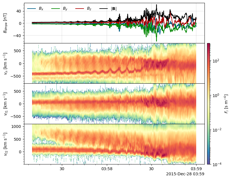
Example to compute and plot reduced ion distributions from FPI

[1]:

%matplotlib inline

import matplotlib.pyplot as plt
import numpy as np

from pyrfu import mms, pyrf
from pyrfu.plot import plot_spectr, plot_line, use_pyrfu_style

use_pyrfu_style(usetex=True)

Load IGRF coefficients ...

Load data#

Define time interval and spacecraft index#

[2]:

mms.db_init(default="local", local="/Volumes/mms")
tint = ["2015-12-28T03:57:10", "2015-12-28T03:59:00"]
mms_id = 1

[29-Jan-26 16:35:07] INFO: Updating MMS data access configuration in /Users/louisr/Dropbox/Documents/irfu-python/.venv/lib/python3.14/site-packages/pyrfu/mms/config.json...
[29-Jan-26 16:35:07] INFO: Updating MMS SDC credentials in /Users/louisr/.config/python_keyring...

[3]:

b_dmpa = mms.get_data("b_dmpa_fgm_brst_l2", tint, mms_id)

[29-Jan-26 16:35:07] INFO: Loading mms1_fgm_b_dmpa_brst_l2...

Get spacecraft attitude (for conversion between Geocentric Solar Ecliptic to spacecrat coordinates)#

[4]:

defatt = mms.load_ancillary("defatt", tint, mms_id)

[29-Jan-26 16:35:08] INFO: Loading ancillary defatt files...

Get the ion velocity distribution skymap and the uncertainties (\(\delta f / f = 1/\sqrt{n}\) with \(n\) the number of counts)#

[5]:

vdf_i = mms.get_data("pdi_fpi_brst_l2", tint, mms_id)
vdf_i_err = mms.get_data("pderri_fpi_brst_l2", tint, mms_id)

[29-Jan-26 16:35:11] INFO: Loading mms1_dis_dist_brst...
[29-Jan-26 16:35:12] INFO: Loading mms1_dis_disterr_brst...

Ignore phase-space density for one count level (also makes function faster)#

[6]:

vdf_i.data.data[vdf_i.data.data < 1.1 * vdf_i_err.data.data] = 0.0

Define the coordinates system for projection of the distribution function#

Shock normal vector in GSE (get this from irf_shock_normal or irf_shock_gui)#

[7]:

n_vec = np.array([0.9580, -0.2708, -0.0938])
n_vec /= np.linalg.norm(n_vec)

Upstream magnetic field in GSE#

[8]:

b_u = [-1.0948, -2.6270, 1.6478]

\(t_2\) vector in GSE (same vectors as in [Johlander et al. 2016, PRL])#

[9]:

t2_vec = np.cross(n_vec, b_u) / np.linalg.norm(np.cross(n_vec, b_u))

\(t_1\) vector in GSE#

[10]:

t1_vec = np.cross(t2_vec, n_vec)

Construct the time series for \(n\), \(t_1\), and \(t_2\)#

[11]:

n_t = len(b_dmpa.time.data)
n_gse = pyrf.ts_vec_xyz(b_dmpa.time.data, np.tile(n_vec[np.newaxis, :], [n_t, 1]))
t1_gse = pyrf.ts_vec_xyz(b_dmpa.time.data, np.tile(t1_vec[np.newaxis, :], [n_t, 1]))
t2_gse = pyrf.ts_vec_xyz(b_dmpa.time.data, np.tile(t2_vec[np.newaxis, :], [n_t, 1]))

Transform the vectors into spacecraft coordinates using the spacecraft attitude#

[12]:

n_dmpa = mms.dsl2gse(n_gse, defatt, -1)
t1_dmpa = mms.dsl2gse(t1_gse, defatt, -1)
t2_dmpa = mms.dsl2gse(t2_gse, defatt, -1)

Create the transformation matrices from spacecraft coordinates#

[13]:

nt1t2 = np.transpose(np.stack([n_dmpa.data, t1_dmpa.data, t2_dmpa.data]), [1, 2, 0])
nt1t2 = pyrf.ts_tensor_xyz(b_dmpa.time.data, nt1t2)

t1t2n = np.transpose(np.stack([t1_dmpa.data, t2_dmpa.data, n_dmpa.data]), [1, 2, 0])
t1t2n = pyrf.ts_tensor_xyz(b_dmpa.time.data, t1t2n)

t2nt1 = np.transpose(np.stack([t2_dmpa.data, n_dmpa.data, t1_dmpa.data]), [1, 2, 0])
t2nt1 = pyrf.ts_tensor_xyz(b_dmpa.time.data, t2nt1)

Define velocity grid along the three vectors#

[14]:

vn_lim = np.array([-800.0, 800.0], dtype=np.float64)
vt1_lim = vn_lim
vt2_lim = vn_lim + 300.0

vg_1d_n = 1e3 * np.linspace(vn_lim[0], vn_lim[1], 100)
vg_1d_t1 = 1e3 * np.linspace(vt1_lim[0], vt1_lim[1], 100)
vg_1d_t2 = 1e3 * np.linspace(vt2_lim[0], vt2_lim[1], 100)

Reduce distribution along the three vectors#

[15]:

n_mc = 200

f1dn = mms.reduce(vdf_i, projection_dim="1d", xyz=nt1t2, n_mc=n_mc, vg=vg_1d_n)
f1dt1 = mms.reduce(vdf_i, projection_dim="1d", xyz=t1t2n, n_mc=n_mc, vg=vg_1d_t1)
f1dt2 = mms.reduce(vdf_i, projection_dim="1d", xyz=t2nt1, n_mc=n_mc, vg=vg_1d_t2)

100%|████████████████████| 733/733 [00:06<00:00, 117.45it/s]
100%|████████████████████| 733/733 [00:05<00:00, 136.36it/s]
100%|████████████████████| 733/733 [00:05<00:00, 144.65it/s]

Plot#

[16]:

f, axs = plt.subplots(4, sharex="all", figsize=(9, 6.5))
f.subplots_adjust(hspace=0.0, left=0.15, right=0.85, bottom=0.08, top=0.95)

plot_line(axs[0], b_dmpa)
plot_line(axs[0], pyrf.norm(b_dmpa), color="k")
axs[0].legend([r"$B_{x}$", r"$B_{y}$", r"$B_{z}$", r"$|\mathbf{B}|$"], ncol=4)
axs[0].set_ylabel("$B_{dmpa}~[\mathrm{nT}]$")

axs[1], cax1 = plot_spectr(
    axs[1], f1dn, cscale="log", clim=[1e-4, 1e3], cmap="Spectral_r"
)
axs[1].set_ylim(vn_lim)
axs[1].set_ylabel("$v_n~[\\mathrm{km}~\\mathrm{s}^{-1}]$")
axs[1].set_yticks([-500.0, 0.0, 500.0])

axs[2] = plot_spectr(
    axs[2], f1dt1, cscale="log", clim=[1e-4, 1e3], colorbar="none", cmap="Spectral_r"
)
axs[2].set_ylim(vt1_lim)
axs[2].set_ylabel("$v_{t1}~[\\mathrm{km}~\\mathrm{s}^{-1}]$")
axs[2].set_yticks([-500.0, 0.0, 500.0])

axs[3] = plot_spectr(
    axs[3], f1dt2, cscale="log", clim=[1e-4, 1e3], colorbar="none", cmap="Spectral_r"
)
axs[3].set_ylim(vt2_lim)
axs[3].set_ylabel("$v_{t2}~[\\mathrm{km}~\\mathrm{s}^{-1}]$")
axs[3].set_yticks([0.0, 500.0, 1000.0])

pos_axs3 = axs[3].get_position()
pos_cax1 = cax1.get_position()
x0 = pos_cax1.x0
y0 = pos_axs3.y0
width = pos_cax1.width
height = pos_cax1.y0 + pos_cax1.height - y0
cax1.set_position([x0, y0, width, height])

cax1.set_ylabel("$F_i~[\\mathrm{s}~\\mathrm{m}^{-4}]$")
f.align_ylabels(axs)

[29-Jan-26 16:35:29] WARNING: <>:7: SyntaxWarning: "\m" is an invalid escape sequence. Such sequences will not work in the future. Did you mean "\\m"? A raw string is also an option.

[29-Jan-26 16:35:29] WARNING: <>:7: SyntaxWarning: "\m" is an invalid escape sequence. Such sequences will not work in the future. Did you mean "\\m"? A raw string is also an option.

[29-Jan-26 16:35:29] WARNING: /var/folders/z6/4tzcn4qs67j8glvrfvkzlkg80000gn/T/ipykernel_79867/2743122119.py:7: SyntaxWarning: "\m" is an invalid escape sequence. Such sequences will not work in the future. Did you mean "\\m"? A raw string is also an option.
  axs[0].set_ylabel("$B_{dmpa}~[\mathrm{nT}]$")

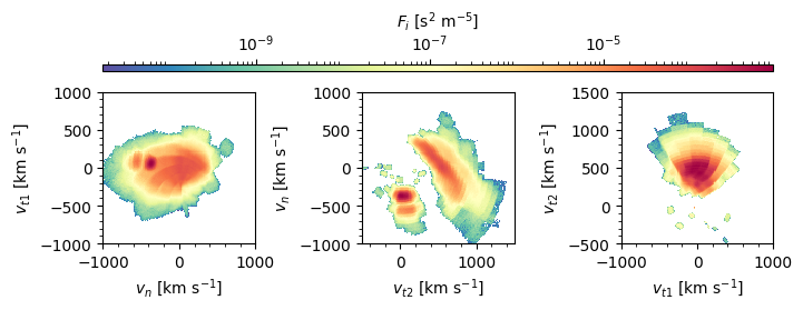
../../_images/examples_01_mms_example_mms_reduced_ion_dist_33_1.png

2D projection of the ion velocity distribution functions#

Define the center time \(\pm 1~\mathrm{s}\) (to average the distributions)#

[17]:

t_2d = np.datetime64("2015-12-28T03:57:40.300")
t_2d = pyrf.extend_tint([t_2d, t_2d], [-1, 1])

Define the velocity grid for 2D projection#

[18]:

vg_2d = np.linspace(-1500, 1500, 200) * 1e3

Reduce ion distributions in 2d planes \((n, t_1)\), \((t_2, n)\), and \((t_1, t_2)\)#

[19]:

f2Dnt1 = mms.reduce(
    pyrf.time_clip(vdf_i, t_2d),
    xyz=nt1t2,
    dim="2d",
    base="cart",
    n_mc=n_mc * 5,
    vg=vg_2d,
)
f2Dt2n = mms.reduce(
    pyrf.time_clip(vdf_i, t_2d),
    xyz=t2nt1,
    dim="2d",
    base="cart",
    n_mc=n_mc * 5,
    vg=vg_2d,
)
f2Dt1t2 = mms.reduce(
    pyrf.time_clip(vdf_i, t_2d),
    xyz=t1t2n,
    dim="2d",
    base="cart",
    n_mc=n_mc * 5,
    vg=vg_2d,
)

100%|███████████████████████| 14/14 [00:00<00:00, 22.85it/s]
100%|███████████████████████| 14/14 [00:00<00:00, 27.26it/s]
100%|███████████████████████| 14/14 [00:00<00:00, 25.67it/s]

Plot#

[20]:

f, axs = plt.subplots(1, 3, figsize=(7, 3.0))
f.subplots_adjust(wspace=0.7, left=0.11, right=0.97, bottom=0.2, top=0.78)
axs[0], cax0 = plot_spectr(
    axs[0], f2Dnt1.mean(axis=0), cscale="log", colorbar="top", cmap="Spectral_r"
)
axs[0].set_xlim([-1e3, 1e3])
axs[0].set_ylim([-1e3, 1e3])
axs[0].set_aspect("equal")
axs[0].set_xlabel("$v_{n}~[\\mathrm{km}~\\mathrm{s}^{-1}]$")
axs[0].set_ylabel("$v_{t1}~[\\mathrm{km}~\\mathrm{s}^{-1}]$")

axs[1] = plot_spectr(
    axs[1], f2Dt2n.mean(axis=0), cscale="log", colorbar="none", cmap="Spectral_r"
)
axs[1].set_xlim([-0.5e3, 1.5e3])
axs[1].set_ylim([-1e3, 1e3])
axs[1].set_aspect("equal")
axs[1].set_xlabel("$v_{t2}~[\\mathrm{km}~\\mathrm{s}^{-1}]$")
axs[1].set_ylabel("$v_{n}~[\\mathrm{km}~\\mathrm{s}^{-1}]$")

axs[2] = plot_spectr(
    axs[2], f2Dt1t2.mean(axis=0), cscale="log", colorbar="none", cmap="Spectral_r"
)
axs[2].set_xlim([-1e3, 1e3])
axs[2].set_ylim([-0.5e3, 1.5e3])
axs[2].set_aspect("equal")
axs[2].set_xlabel("$v_{t1}~[\\mathrm{km}~\\mathrm{s}^{-1}]$")
axs[2].set_ylabel("$v_{t2}~[\\mathrm{km}~\\mathrm{s}^{-1}]$")

pos_axs2 = axs[2].get_position()
pos_cax0 = cax0.get_position()
x0 = pos_cax0.x0
y0 = pos_cax0.y0 - 0.01
width = pos_axs2.x0 + pos_axs2.width - pos_cax0.x0
height = 0.02
cax0.set_position([x0, y0, width, height])

cax0.set_xlabel("$F_i~[\\mathrm{s}^2~\\mathrm{m}^{-5}]$")

[20]:

Text(0.5, 0, '$F_i~[\\mathrm{s}^2~\\mathrm{m}^{-5}]$')

../../_images/examples_01_mms_example_mms_reduced_ion_dist_43_1.png

[ ]:

[ ]: